O(V+E) Complexity in DFS and BFS of a Graph

The Time Complexity for DFS and BFS is O(V+E). We all know that. But what does V+E is actually mean ? Ever noticed Dijkstra also has this V+E in its time complexity = O((V+E)logV). Ever wondered why ?

Understanding DFS and BFS

Depth First Search and Breadth First Search are two graph traversal algorithms. While DFS explores the graph recursively, BFS explores the graph level by level. Let’s see the two algorithms:

DFS

1. Pick an unvisited node.

• Mark the node as visited.
• Pick an unvisited neighbor and recursively explore it.
• Do previous steps for the neighbor.

2. Repeat step 1 till all nodes are visited.

Due to recursion DFS internally uses a stack. The stack size can grow depending on the longest path of a graph.

Here’s the implementation of DFS:

# Using adjacency list
def dfs(self, size, graph):
  visited = [False]*size

  # Recursively explore unvisited neighbors
  # of the node.
  def recursion(node):
    neighbours = graph[node]

    for nei in neighbours:
      if not visited[nei]:
        visited[nei] = True
        recursion(nei)

  # Try DFS for all nodes, this ensures nodes
  # which are not connected to the graph are
  # also explored.
  for node in range(size):
    if not visited[node]:
      visited[node] = True
      recursion(node)

BFS

1. Pick an unvisited node and enqueue it in a queue.

• Deque a node from the queue. Mark the node as visited.
• Append all unvisited neighbors of the node in the queue.
• Repeat the previous steps until the queue is empty.

2. Repeat step 1 till all nodes are visited.

BFS uses a queue to explore the graph. The queue size depends on the connectivity of a graph, for a strongly connected graph the queue size can go upto the number of vertices.

Here’s the implementation of BFS:

def bfs(self, size, graph):
  visited = [False]*size

  def traverse(node):
    queue = [node]
    visited[node] = True

    while len(queue) > 0:
      curr = queue.pop(0)

      print(curr)

      for nei in graph[curr]:
        if not visited[nei]:
          visited[curr] = True
          queue.append(nei)

  # Try BFS for all nodes, this ensures nodes
  # which are not connected to the graph are
  # also explored.
  for node in range(size):
    if not visited[node]:
      visited[node] = True
      traverse(node)

DFS and BFS are quite straightforward to understand. Their TC is where things gets interesting. To understand the TC of DFS and BFS we’ll first understand what is a sparse graph and a dense graph.

Sparse graph

A graph is sparse when the number of edges are far less than the maximum number of edges a graph can have. As an example let’s take a graph where number of edges is half the max number of edges:

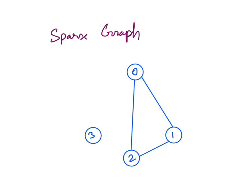
The above graph has 3 edges, the max number of edges the graph can have is 6 edges hence this is a sparse graph. Also note that node 3 is disconnected from the graph.

TC analysis for Sparse graph

To understand TC analysis for sparse graph lets run DFS on the previous example. We start the DFS from node 0:

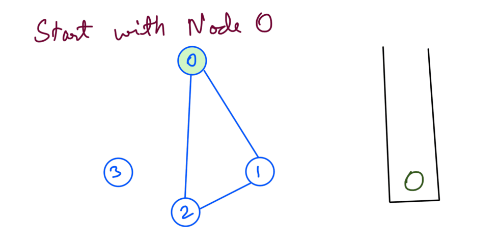
From node 0 we explore node 1 recursively:

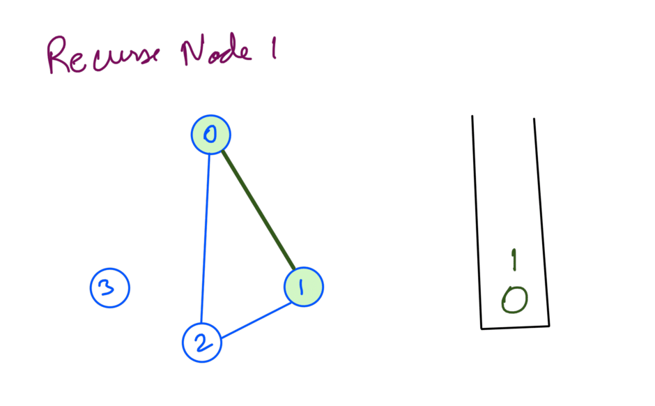
And from node 1 we explore node 2 recursively:

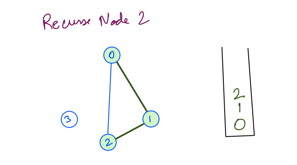
Node 2 has no unvisited neighbors so we backtrack from node 2:

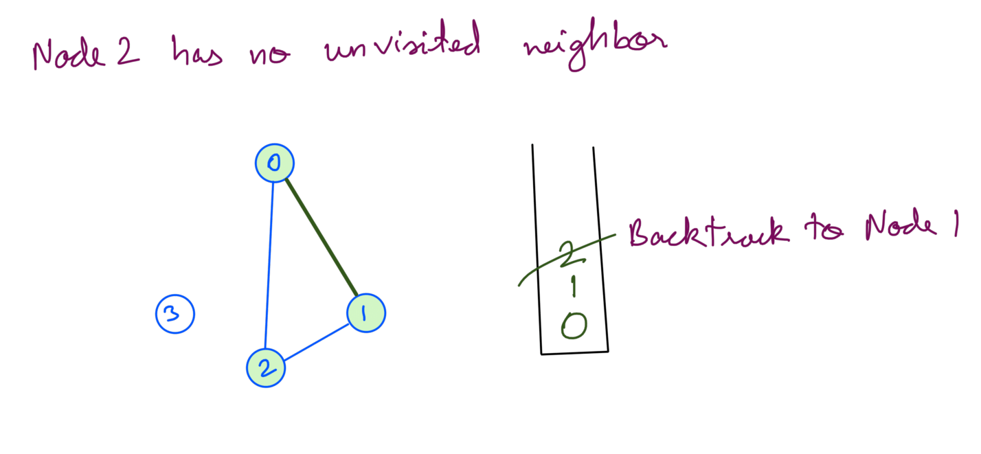
Similarly we backtrack from node 1 and node 0:

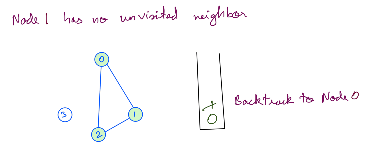
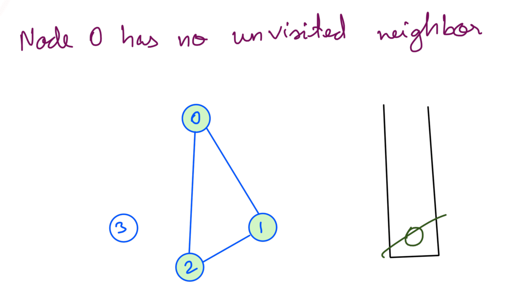
At this point we check if there are any unvisited nodes left. Node 3 is still unvisited so we recurse with Node 3:

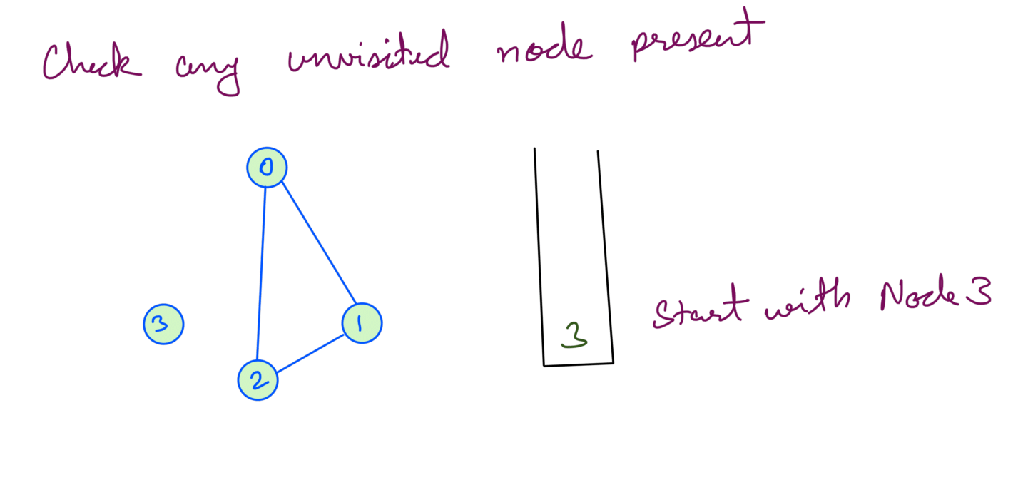
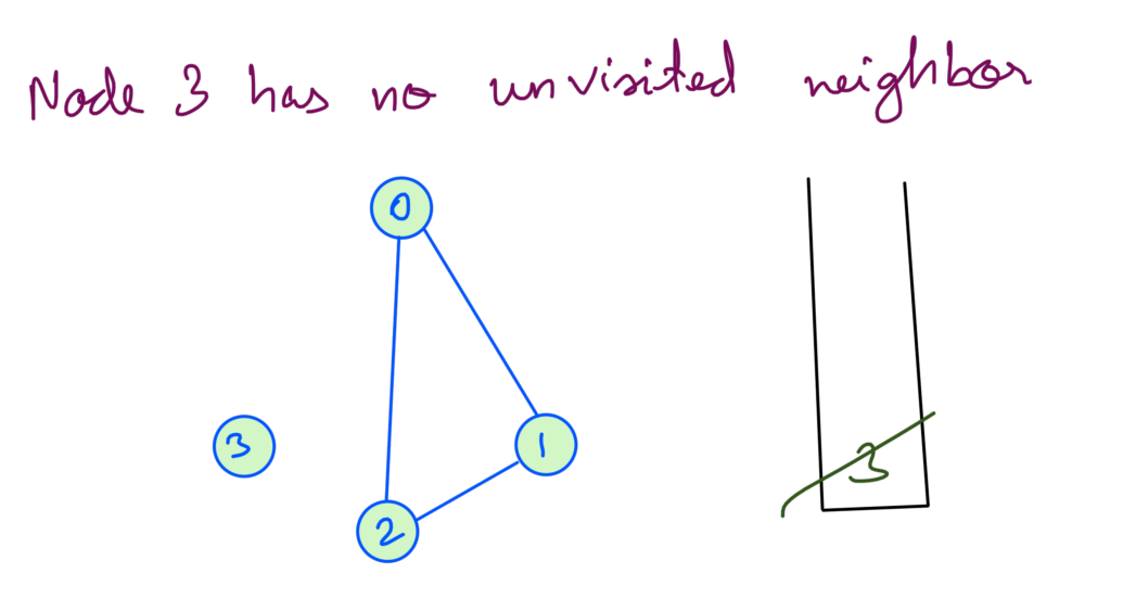
Now we’ve explored all the nodes.

We can see from the above dry run that we’re exploring each node once, as there not many edges we can conclude that the TC depends on V in case of sparse graphs.

Dense graph

A graph is dense when the number of edges are much closer to the maximum number of edges a graph can have. As an example let’s take a graph where number of edges is equal to the max number of edges:

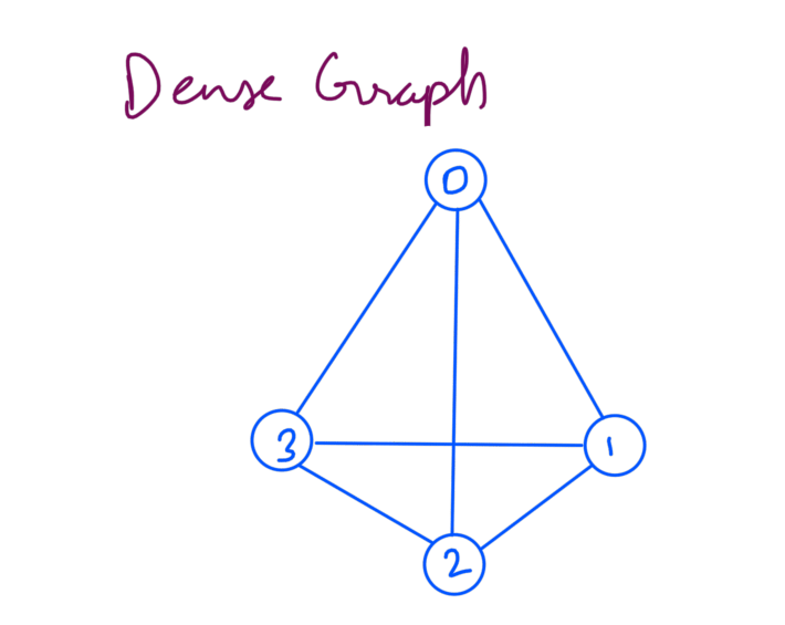
The above graph has 6 edges which is the max number of edges for graph with 4 vertices. To calculate the max number of edges we can use the combinatorics, the max number of edges in a graph with V vertices is equal to the number of ways of selecting 2 vertices = nC2 = V(V-1)/2.

TC analysis for Dense graph

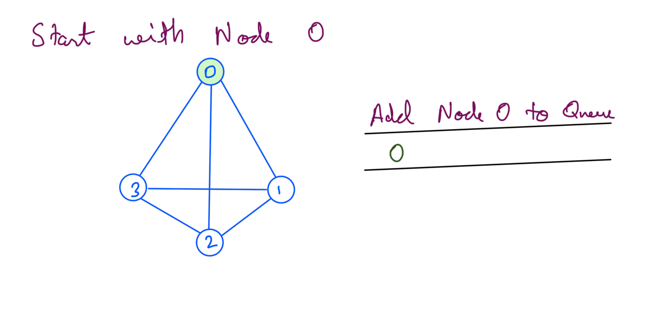
To understand TC analysis for sparse graph we’re going to run BFS this time. We start the BFS from node 0:

We add unvisited neighbors of node 0 to the queue:

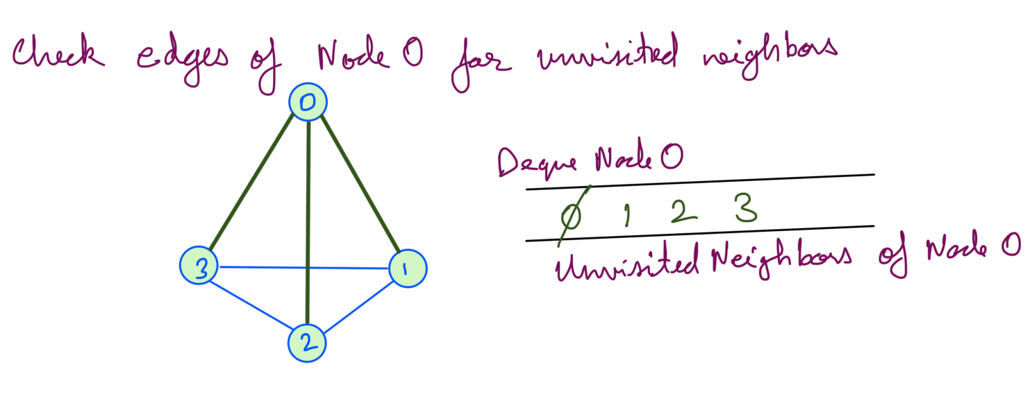
Then we deque node 1. As node 1 has no unvisited we don’t add anything in the queue:

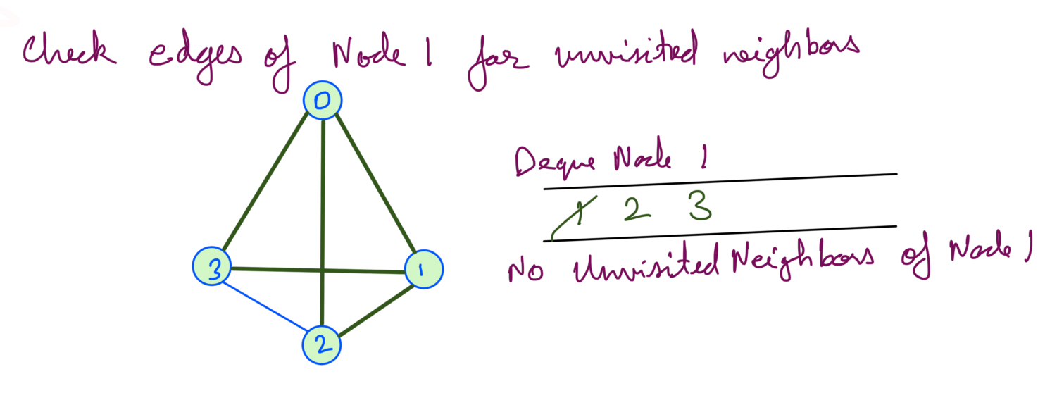
Then we deque node 2 and node 3. Both node 2 and node 3 has no unvisited neighbors so we don’t add anything in the queue:

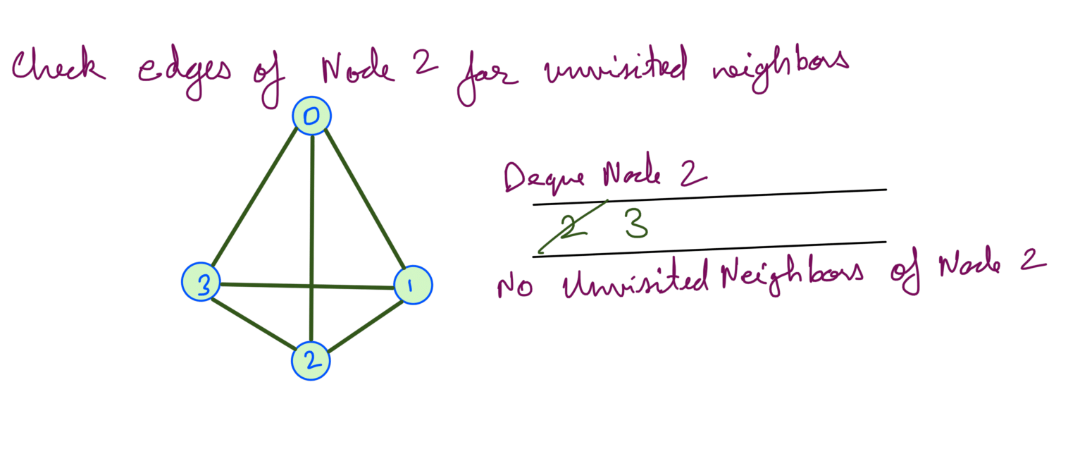
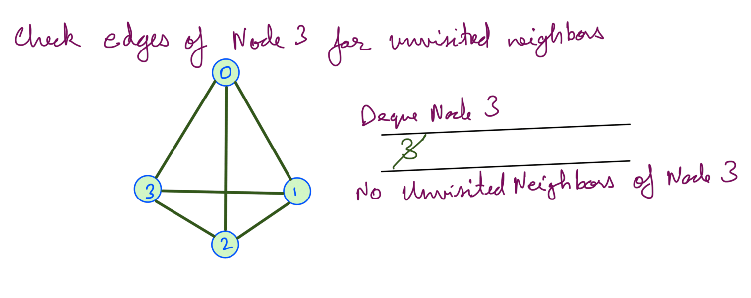
Now we’ve explored all the nodes.

We can see from the above dry run that although we’re exploring each node once, we’re also exploring all the edges at each node. As this is a dense graph the number edges E becomes significant and we cannot ignore it as we did for sparse graph.

Since in an undirected graph an edge will be seen 2 times, once from each node the edge connects so total time will be 2E.

Meaning of V+E in Graphs

Going through the sparse and dense graph examples we understood that the TC of graphs depends not just on the vertices but also on the connectivity of the graph.

When connectivity is fairly less, the TC tends to depend on V and when the connectivity is high, the TC tends to depend on E.

Keeping those two observations in mind, the TC of DFS and BFS will be:

TC = max(V,E)
   = O(V+E)