Dijkstra - Single Source Shortest Path

Dijkstra is a Greedy algorithm to find the shortest path in a graph from a single source.

Let’s take a weighted a graph as below:

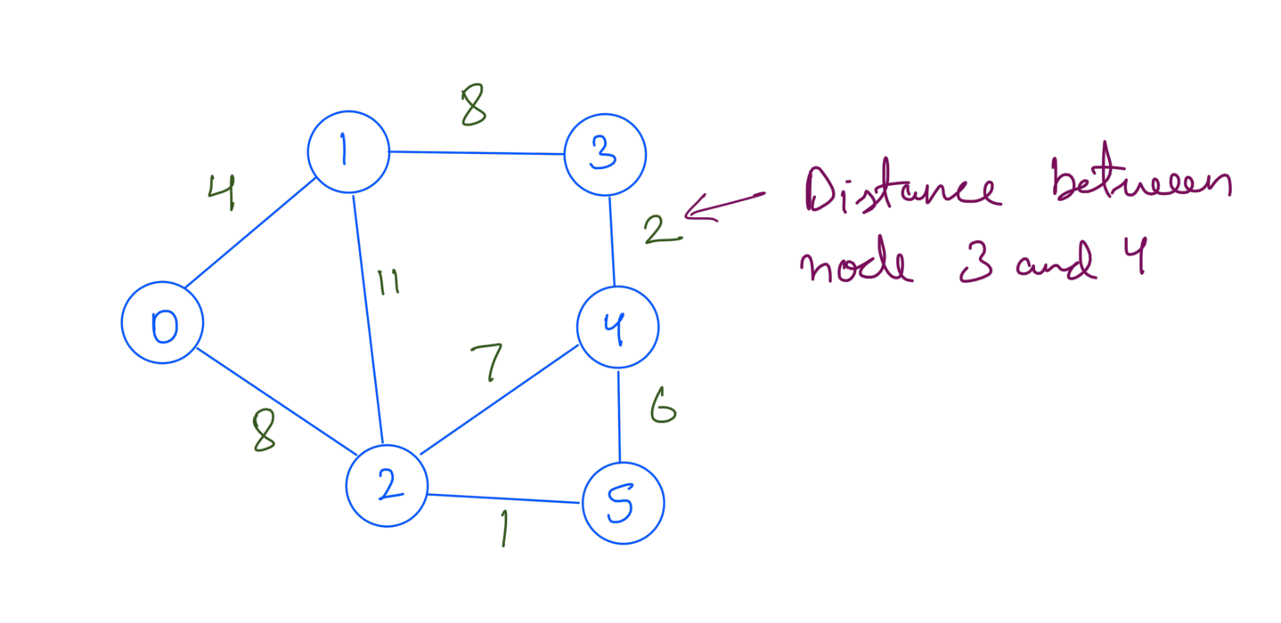
We’ll take 0 as the source. Shortest path from source 0 to node 4 will go through node 1 and node 3:

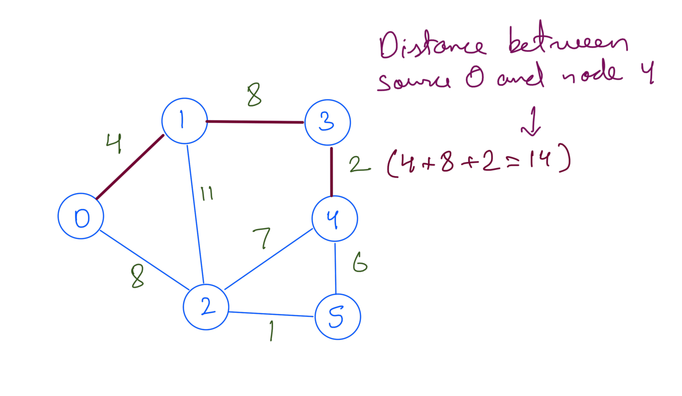
Similarly we’ve to find the shortest path from the source 0 to every node.

How does Dijkstra finds this ?

Understanding Dijkstra

Dijkstra like any other Greedy algorithm finds the next most optimum path at each step. We do this by taking the nodes with minimum distance from source 0 at each step. Here’s how it looks like:

• Initialize
  • a dist array which holds the distance from src 0 to that node.
  • a heap h to hold the minimum distance from src 0.
  • a set processed which holds the nodes which has been processed.
• Add src 0 to heap by pushing (0,0) which is (node’s distance from 0, node’s identifier).
• Until heap is not empty do following:
  • Pop the node with minimum distance(node_distance) from src.
  • Update dist array if node_distance < dist[node].
  • Mark node as processed.
  • for each neighbor of node which is not processed, push (neighbors_distance + dist[node], neighbor) into heap h.
• Return dist.

Running the above steps on the example graph gives us the shortest path from src 0:

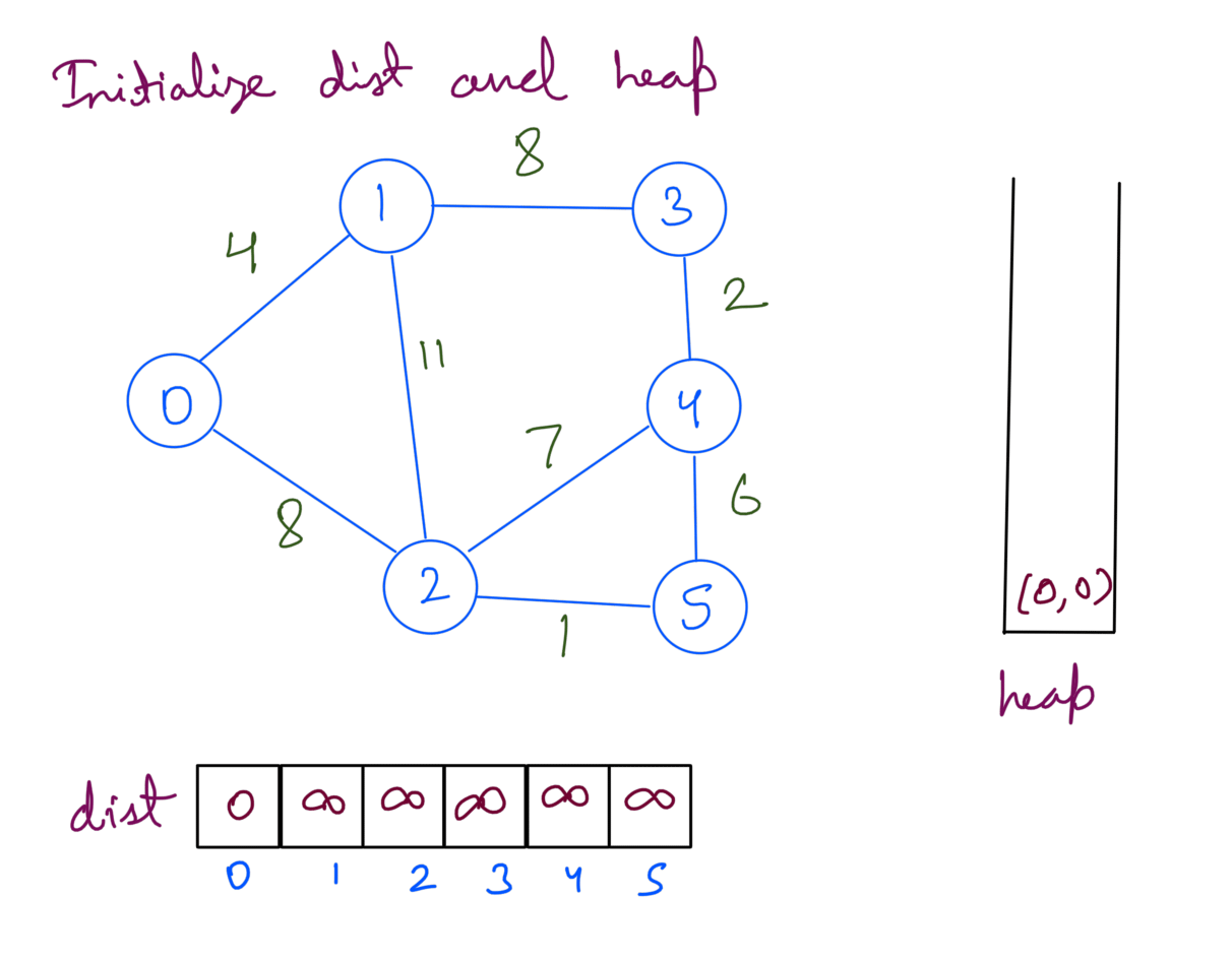
Firstly we initialize the heap, dist arry.

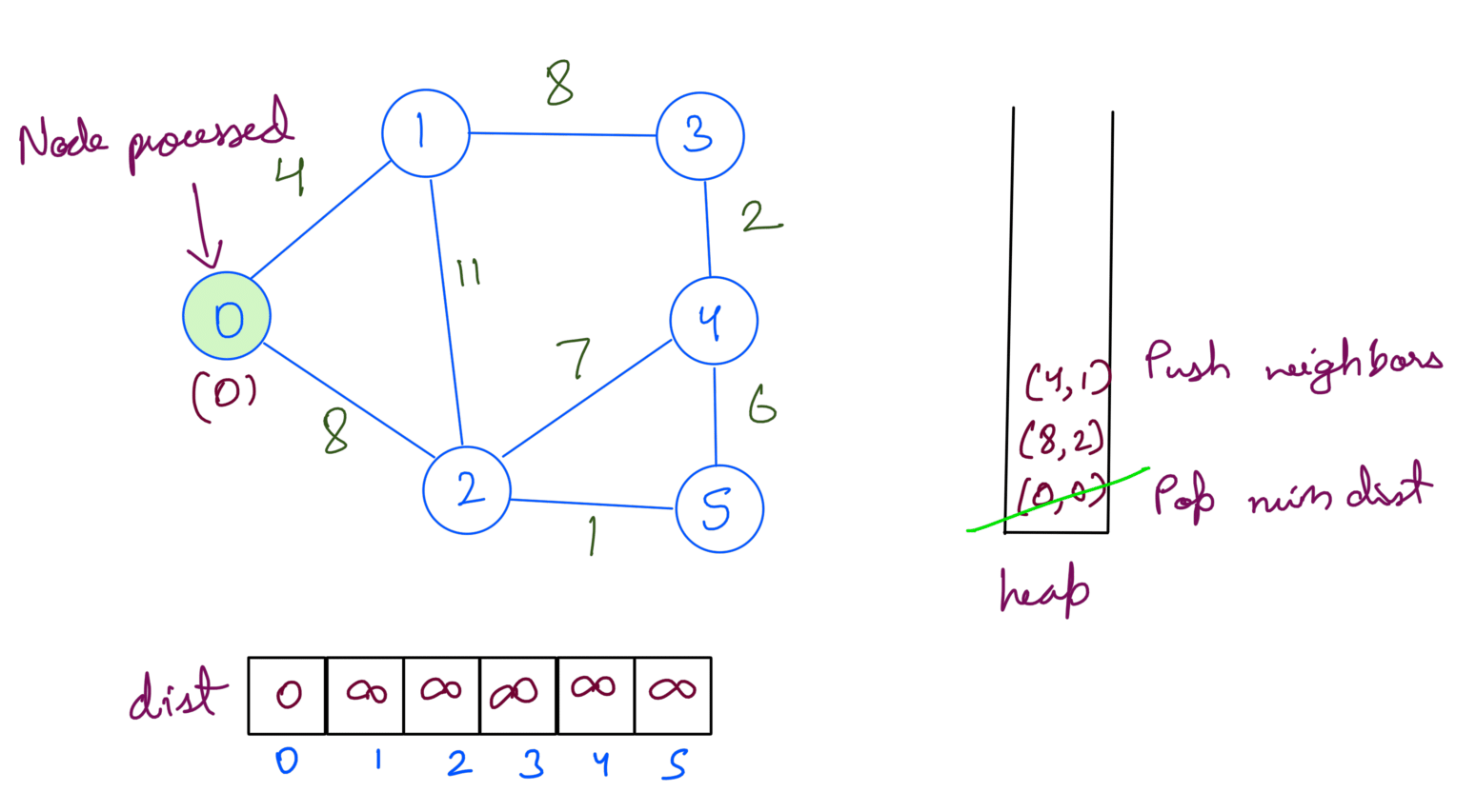
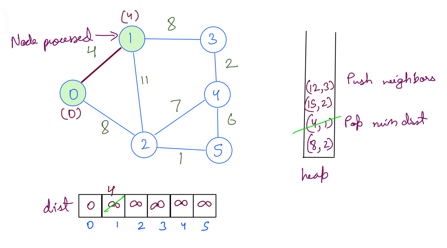
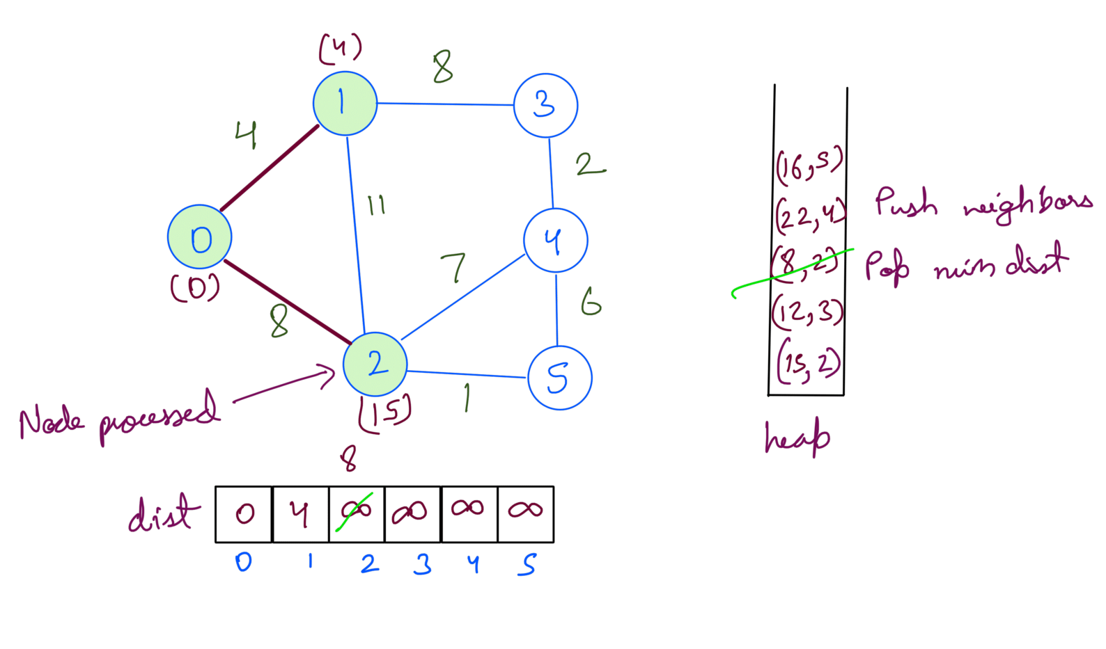
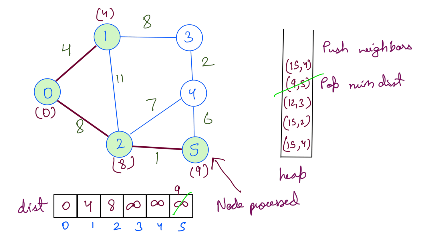
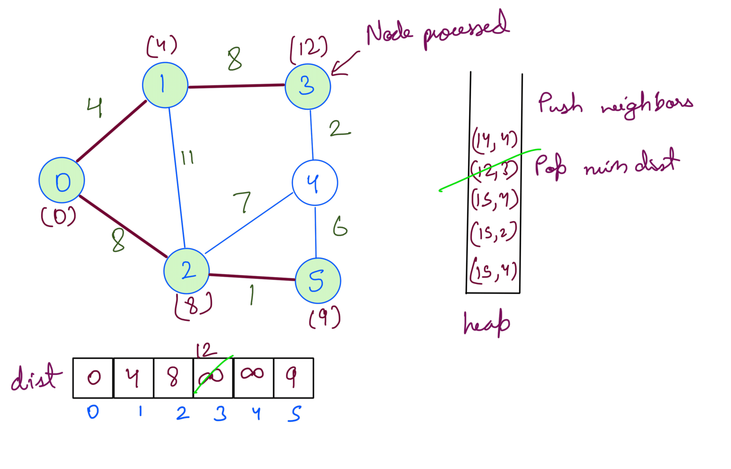
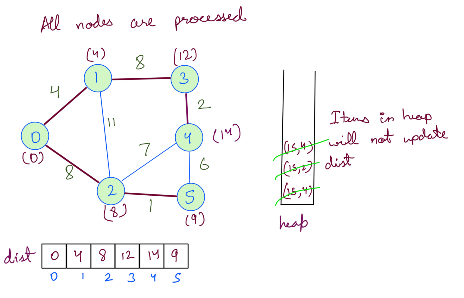
Then we extract min dist node from heap. We update the dist array and push the node’s neighbors into the heap. We repeat the process until the heap is empty. 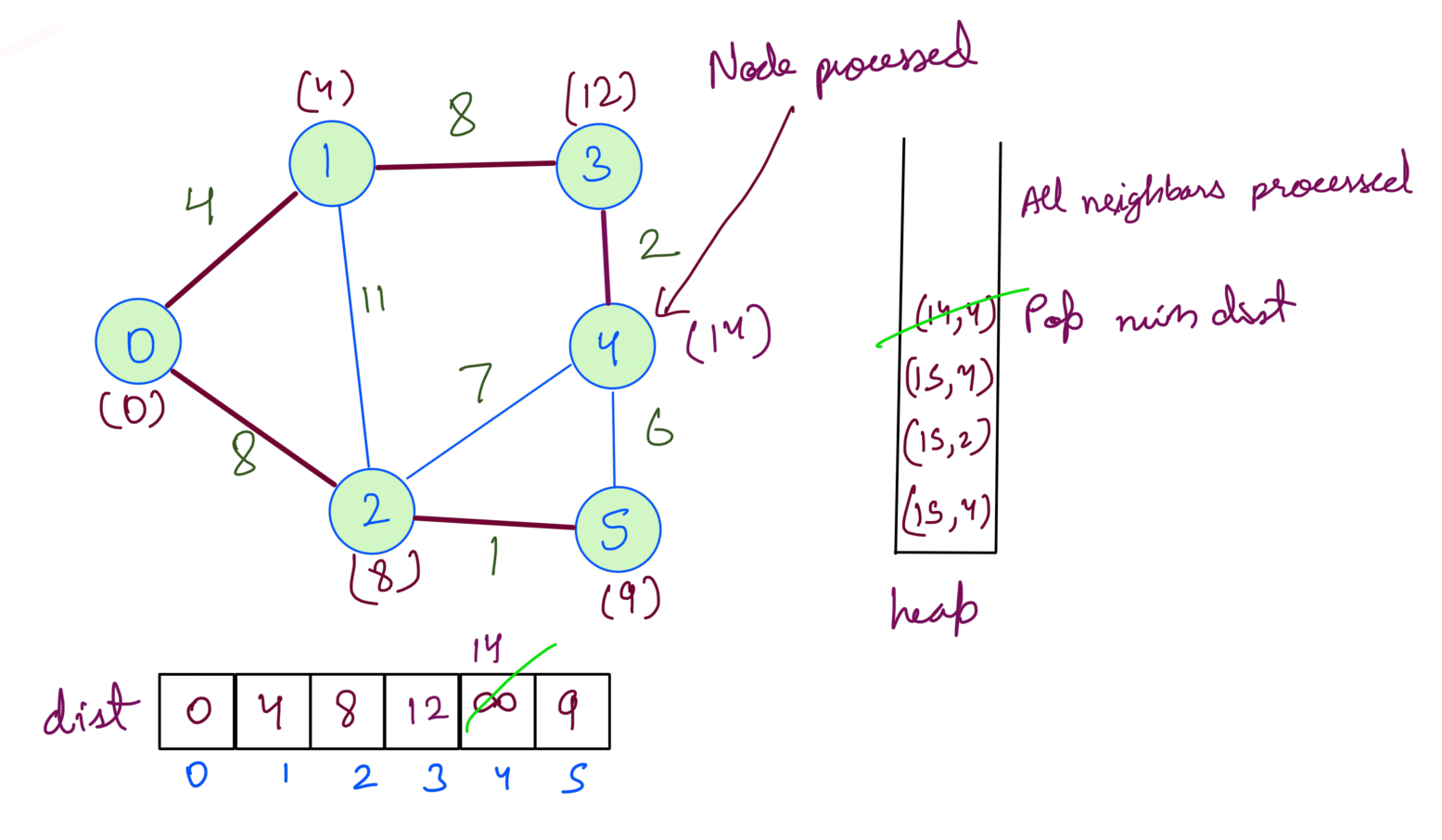At this point, we’ve processed all the nodes. If we check the heap we’ll notice that the distances for the nodes are already at min in the dist array. Processing will not change the answer but since we’re checking for heap being empty we’ll pop them one by one.

Implementation of the pseudocode is:

import heapq
# graph is represented as an adjacency list
# {
#   0: [(1,3), (2,6)]
#   1: [(0,5), (3,2)]
#   ...
# }
def dijkstra(graph, src, V):
  dist = [float('inf')] * V
  dist[src] = 0

  h = [(0,src)]

  visited = set()
  visited.add(0)

  heapq.heapify(h)

  while len(h) > 0:
    weight, dest = heapq.heappop(h)
    visited.add(dest)

    dist[dest] = min(weight, dist[dest])

    for nei, nei_weight in graph[vertex]:
      if nei not in visited:
        heapq.heappush(h, (dist[vertex] + nei_weight, nei))

  return dist

Time Complexity Analysis

To understand the Time Complexity let’s look at what we’re doing:

• We’re going through each node and checking all its edges.
• Each time we do this we’re doing a heap operation.

These two steps depends on the graph’s edges and nodes, and the size heap.

We can easily see that the size of the heap can go upto number of edges in the graph.

What about the graph’s edges and nodes ? To answer that we’ve consider two kinds of graphs - dense graph and sparse graph.

TC for sparse graph

In case of a sparse graph let’s say there is one edge for each vertex, we’ll be pushing and popping once for each vertex. So the TC for sparse graph in worst case will depend on number of vertices.

TC(sparse graph) = O(VlogE)

TC for dense graph

In case of a dense graph though we’ll push all the edges and pop them. So the TC for dense graph will depend on number of edges which will more than the vertices.

TC(dense graph) = O(ElogE)

Overall TC

Taking the 2 cases into consideration the TC will be:

TC = TC(sparse graph) + TC(dense graph)
   = O(VlogE) + O(ElogE)
   = O((V+E)logE)

We can further optimize this by using decreaseKey to update the dist in the heap instead of inserting it again and again, if we’re only updating the min distance for each vertex then the heap can have V items in worst case. Then the TC for Dijkstra becomes O((E+V)logV).

Dijkstra with decrease key

Remember the last step of the dry run we did for our graph example. These items are duplicates for Node 2 and Node 4. They’ll not affect the dist array but we still pop them from heap since we do the steps until heap is empty.

We can avoid having duplicates by updating the value for the node itself in the heap. This will mean the heap will now have atmost V items which changes the TC to O((E+V)logV).

# TC with decrease key
TC = O((E+V)logV)

Dijkstra doesn’t work with Negative edges

Dijkstra doesn’t work with graphs having negative edges because Dijkstra is a Greedy algorithm. If a graph has negative edges then we’ve to consider other paths to reach a node which might have a negative edge and can give us a minimum distance path.

Here’s an example graph with negative edge 1-2:

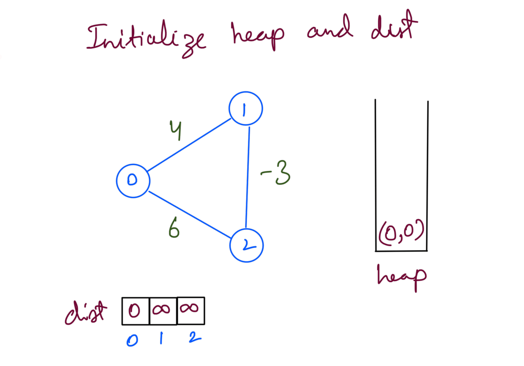
We first process the src 0 which adds neighbor 1 with distance 4:

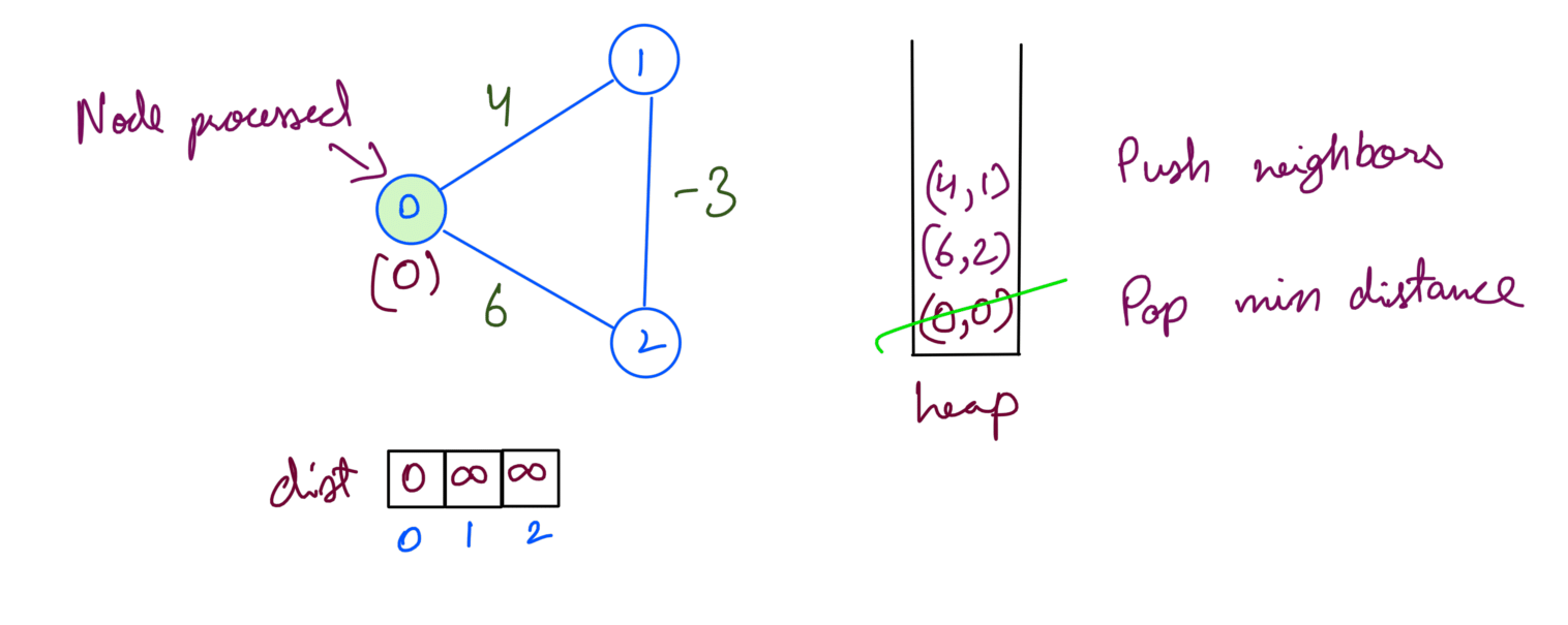
Then we process node 1 which adds neighbor 2 with distance 1. Node 1’s min dist is now 4:

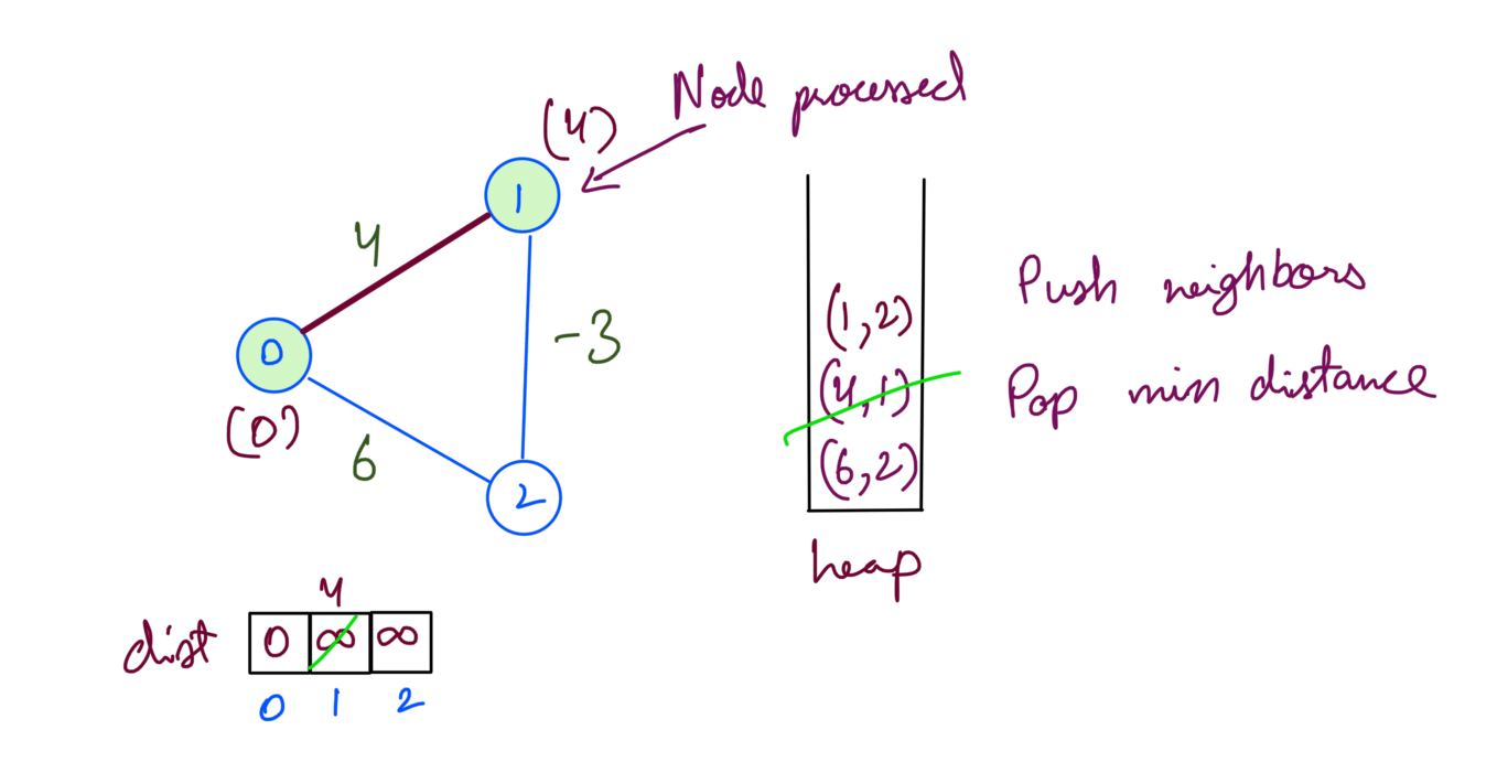
Then we process node 2 which adds no neighbor. Node 2’s min dist is now 1:

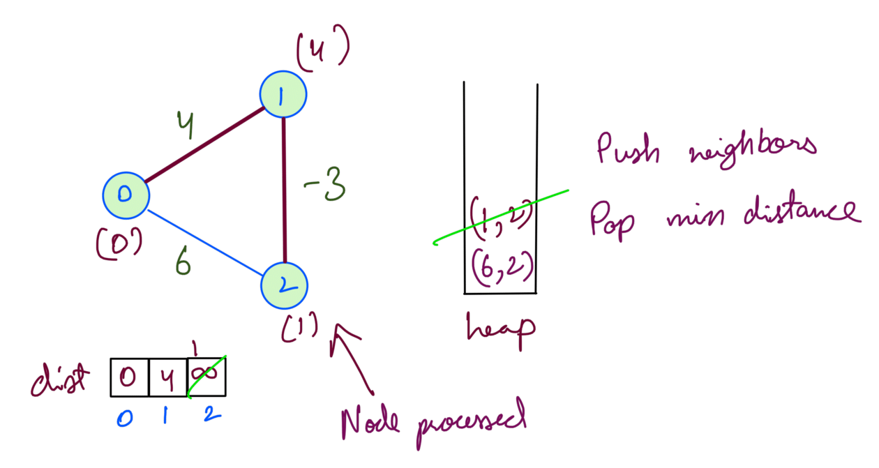
We’ve now processed all nodes. (6,2) will not affect node 2 since we’ve already 1 as the min distance. Dijkstra being a Greedy algo opted for the most optimum path at each step. However the distance for Node 1 is actually 3. Consider the path 0-2-1 containing the negative edge which has distance (6+(-3)) = 3.

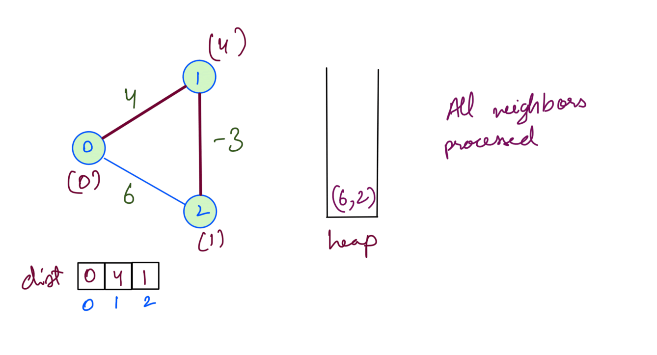
As we have seen for a graph with negative edges we cannot take the most optimum path at each step, we’ve to consider different paths to a node to find the minimum distance.

And that’s why Dijkstra doesn’t work because it’s a Greedy algorithm.