Problem Statement
Given a 2D matrix cost[][] of size MxN where cost[i][j] represents the cost of passing through cell[i][j]. Total cost of reaching a particular cell is the sum of costs of all cells in that path(including the start and end cell). We are allowed to move downward or rightward i.e. from cell[i][j] we can go to cell[i][j+1] or cell[i+1][j].
Find the min cost of moving from cell top left (0, 0) to bottom right (M-1, N-1).
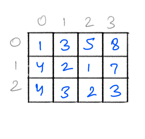
Understanding the Problem
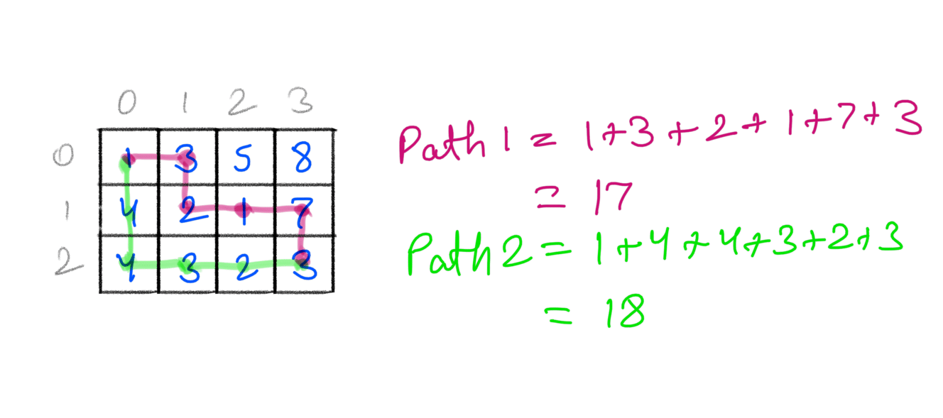
The problems asks us to find a path whose cost is minimum. There are many paths from (0,0) to (M-1, N-1), here are 2 such paths we can take:
Taking the path 1 costs us 17, while taking path 2 costs us 18. There are many such paths.
The most optimal path costs us 12:
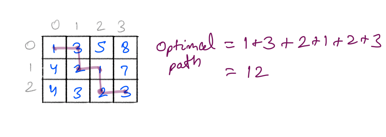
Looking at the examples we can say that if we identify all such problems, we can get the path with the min cost. How to find all possible paths ?
Recursion Top Down Approach
In the given cost matrix, each cell(i,j) can be reached from cell(i-1,j) and cell(i,j-1). Keeping that in mind all the possible paths will be:
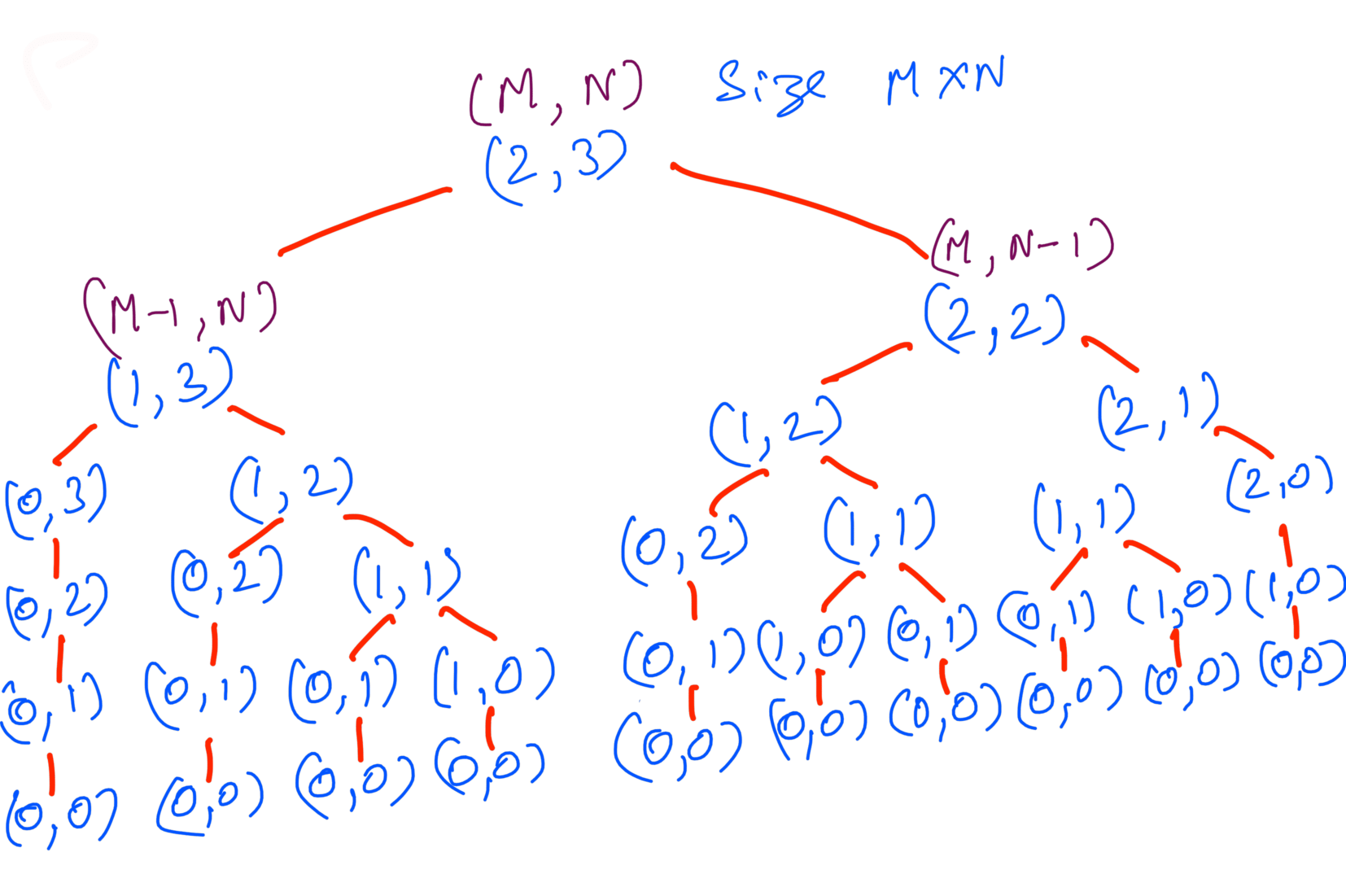
To find the min cost among all the possible paths we’ve to find the min cost at each cell(i,j). As cell[i][j] can be reached either from above or left cell, the min cost for cell(i,j) is:
mincost(i,j) = min(mincost(i-1,j), mincost(i,j-1)) + cost[i][j]
Using recursion our implementation will look like:
def min_path_cost(cost, M, N):
  if M == 0 and N == 0:
    return cost[0][0]

  # First Row
  if M == 0:
    return cost[M][N-1] + cost[0][N]

  # First Column
  if N == 0:
    return cost[M-1][N] + cost[M][0]

  return min(cost[M][N-1], cost[M-1][N]) + cost[M][N]
To calculate the time complexity let’s analyze the above code. We’re calling the function recursively and at each call we’re making atmost two more calls. This is also apparent in the all possible paths figure. If we assume the height of the call tree to be h in that then the total number of calls will be:
TC  = 2^0 + 2^1 + 2^2 ...... + 2^(h-1)
    = 2^0(2^h-1)/(2-1) # Using GP summation
    = 2^h-1
    = O(2^h)
The time complexity is exponential. What’s the height of the tree though ? If we look at the call tree, when (M,N) becomes (0,0) that’s when we’ve reached the leaf node. Also we’re decrementing M or N by 1 at each level so the maximum height will be max(M,N). Considering h = max(M,N):
TC  = O(2^(M+N))
    = O(2^N) # if we assume M == N
So the TC is exponential to the matrix dimensions. We can reduce the TC further but let’s talk about Space Complexity.
Space Complexity will be the maximum height the call tree can achieve. Since that’ll be maximum space needed by the call stack. Considering h = max(M,N):
SC  = O(M+N)
    = O(N) # if we assume M == N
Memoization Top Down Approach
If we take a closer look at the all possible paths we’ll see that multiple function calls are recomputed again and again. Here’s one such case:
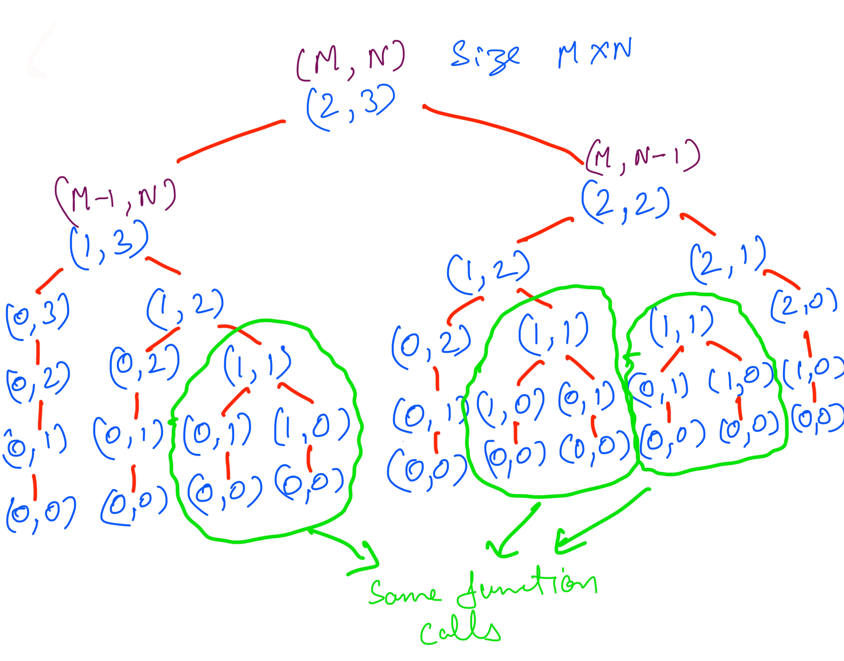
What if we cache these calls instead recomputing it again. That will save a lot of function calls. This is called memoization. Here’s how the call tree will look like with memoization:
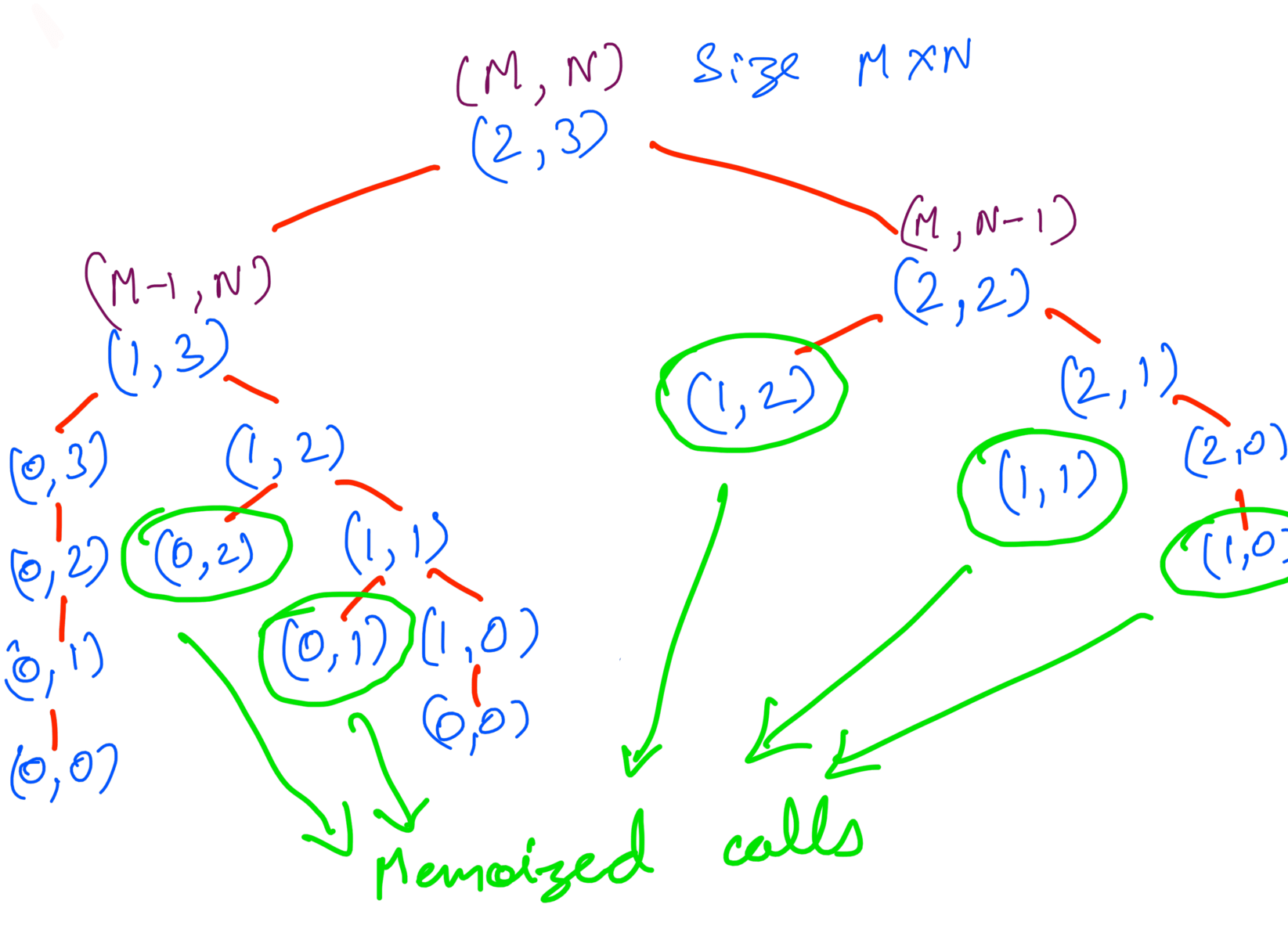
Much better. Implementing memoization is same as recursive implementation. The only difference being we’ll cache the function calls and if we’ve already computed a particular call we’ll use the cache instead of calling it again.
# cache to memoize function calls
mem = [[None for j in range(M)] for i in range(N)]
def min_path_cost(cost, M, N):
  nonlocal mem
  if M == 0 and N == 0:
    return cost[0][0]

  # Reuse the memoized result
  if mem[M][N] is not None:
    return mem[M][N]

  # First Row
  if M == 0:
    mem[M][N] = cost[M][N-1] + cost[0][N]
  # First Column
  elif N == 0:
    mem[M][N] = cost[M-1][N] + cost[M][0]
  else:
    mem[M][N] = min(cost[M][N-1], cost[M-1][N]) + cost[M][N]

  return mem[M][N]
What’s the Time Complexity for the memoized approach ? If we look at the memoized call tree we can see that we’re only computing the all the possible (M,N) values once. And the total possible values for (M,N) are MxN.
TC  = O(MN)
    = O(N^2) # if M == N
That’s drastic improvement from the previous approach. What about Space Complexity ?
Looking at the memoized call tree the maximum call stack will remain the same max(M,N). However additionally we’re also using the mem array which takes O(MN) space. Considering both of them:
TC  = O(M+N) + O(MN)
    = O(MN)
    = O(N^2) # if M == N
Bottom Up Approach
In the previous approaches we’re looking at the problem recursively. We started with (M,N) and let recursion solve it until we reached (0,0). In a sense we’re going from larger values to smaller ones, this is called top down.
Another way to look at it is solving for smaller values like (0,0) then (1,0) then (0,1) so on and building up till we compute for (M,N). If we look at the memoized call tree we’re computing values from bottom till we reach (M,N).
We’ll reuse the mem 2D array we used in memoized approach. We’ll fill that up from (0,0) to (M,N). Here’s a dry run for it:
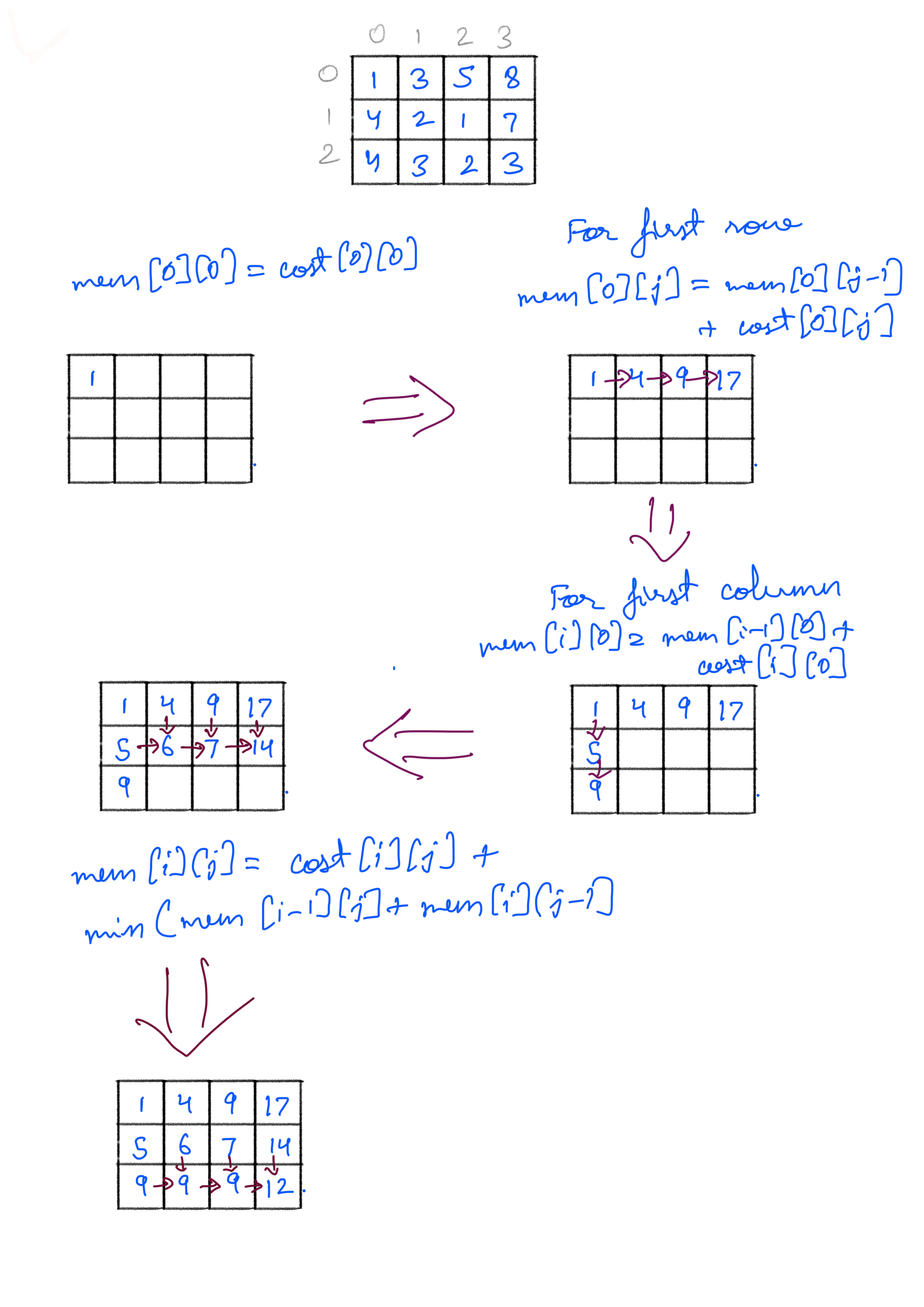
We can implement this iteratively:
def min_path_cost(cost, M, N):
  if M == 0 and N == 0:
    return cost[0][0]

  mem = [[0 for j in range(M)] for i in range(N)]

  mem[0][0] = cost[0][0]
  # First Row
  for j in range(1,N):
    mem[0][j] = mem[0][j-1] + cost[0][j]

  # First Column
  for i in range(1,M):
    mem[i][0] = mem[i-1][0] + cost[i][0]

  for i in range(1,M):
    for j in range(1,N):
      mem[i][j] = cost[i][j] + min(mem[i-1][j], mem[i][j-1])

  return mem[M-1][N-1]
Calculating Time Complexity is fairly simple here. The outer loop takes M time and the inner loop takes N, thus total Time Complexity is MxN.
TC = O(MN)
The Space Complexity same as memoized approach except bottom up being iterative approach we’re not using the call stack. So O(M+N) is not needed here.
SC = O(MN)
We can reduce the Space Complexity to O(1) if we’re allowed to modify the original matrix. In that case we directly use cost matrix as the memoized array.